Retrieving members of parliament

In this post we delve into the get_mp() function and the parameters you can specify to query for more specific information. The get_mp() function has the following arguments:

• selection: options are “current”, “former” or “date”
  • when selecting “date”, “date_at” should be added as “YYYY-MM-DD”
• fact: options are “bio”, “career”, “education”, “presences_commissions”, “presences_plenary”, “political_info”, and “raw”
• use_parallel: Boolean of which the default value is set to TRUE, select FALSE in case you do not have multiple workers to speed up the calls made

To retrieve the demographics of the MPs currently in parliament (same as default), we specify the following: selection="current" and fact="bio". Note that you can each time store the data frame in your R-environment by including the following <- name data frame. This has the benefit of storing the data in a table containing rows and columns that you can use for further data manipulation and analysis.

mp_bio <- get_mp(selection="current"
                , fact="bio") 
mp_bio

The result of our query is a data frame with 124 observations, the exact number of MPs currently in office, and their demographics. You will see that the data frame is successfully stored under the tab ‘Environment’. This is how the data frame looks like:

You can, for instance, check the distribution of men and women in parliament. We make use of the pipe operator %>% (which lets you pass an interim result onto the next function) and the data manipulation options from the dplyr package. To count observations by group, we use group_by() and tally(). You can find more information on how to use dplyr here.

mp_bio %>%
  group_by(geslacht) %>%
  tally()

Example 2 - Extracting demographics at specific dates

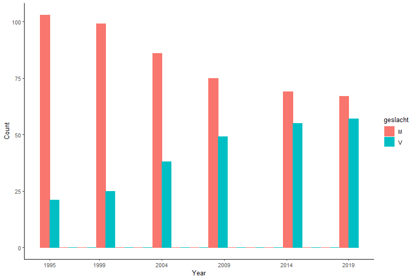
So let’s take this a step further and analyze whether the number of women in parliament has grown throughout the years. To do so, we will extract the demographics of MPs from past legislatures (from 1995 onwards). We make use of the get_legislatures() function to identify the starting dates of each legislature.

get_legislatures()

Next, we specify the exact date from which we wish to collect the MPs’ demographics. Here, we opt for 01/12 of the starting year of each legislature, to make sure all MPs are sworn in. Instead of selection="current", we now fill in selection="date"and add the date_at="YYYY-MM-DD" argument in the the get_mp() function.

mp_bio_1995 <- get_mp(selection="date", fact="bio", date_at ="1995-12-01")
mp_bio_1999 <- get_mp(selection="date", fact="bio", date_at ="1999-12-01")
mp_bio_2004 <- get_mp(selection="date", fact="bio", date_at ="2004-12-01")
mp_bio_2009 <- get_mp(selection="date", fact="bio", date_at ="2009-12-01")
mp_bio_2014 <- get_mp(selection="date", fact="bio", date_at ="2014-12-01")
mp_bio_2019 <- get_mp(selection="date", fact="bio", date_at ="2019-12-01")

Now, we will select the relevant columns to answer our question and add a column for year. We again make use of the pipe operator (which lets you pass an interim result onto the next function) and the data manipulation options from the dplyr package (here: select() and add_column()).

mp_bio_1995 %>%
  select(id_mp, geslacht) %>% add_column(year = 1995) -> mp_bio_1995
mp_bio_1999 %>%
  select(id_mp, geslacht) %>% add_column(year = 1999) -> mp_bio_1999
mp_bio_2004 %>%
  select(id_mp, geslacht) %>% add_column(year = 2004) -> mp_bio_2004
mp_bio_2009 %>%
  select(id_mp, geslacht) %>% add_column(year = 2009) -> mp_bio_2009
mp_bio_2014 %>%
  select(id_mp, geslacht) %>% add_column(year = 2014) -> mp_bio_2014
mp_bio_2019 %>%
  select(id_mp, geslacht) %>% add_column(year = 2019) -> mp_bio_2019

Finally, we combine these data frames into a single data frame, making use of rbind(). This function allows to join data frames vertically, in other words, the data frames get pasted below each other.

mp_pastlegis <- rbind(mp_bio_1995, mp_bio_1999, mp_bio_2004, mp_bio_2009, mp_bio_2014, mp_bio_2019) 
mp_pastlegis

This data frame then allows us to answer our research question. Has the number of women MPs grown throughout the years? We opt to plot the results in a histogram, making use of the ggplot package. A good place to start learning about ggplot is here.

plot1 <- ggplot(mp_pastlegis, aes(x = year, fill= geslacht, colour = geslacht), bins = 12) + 
                geom_histogram(binwidth=1.5, position = "dodge") +
                labs(x="Year", y = "Count") + 
                scale_x_continuous(breaks = c(1995, 1999, 2004, 2009, 2014, 2019)) +
                theme_classic() 
plot1

Quick elaboration (advanced)

Above, we present some very elaborate code, but with the advantage of simplicity to intuitively understand it. Here, we do it in a shorter, elegant, but more complex way.

library(lubridate)

leg <- get_legislatures() %>%
  filter(start >= ymd_hms("1995-06-12 22:00:00"))

list <- vector(mode="list", length=length(leg))

for(i in 1:nrow(leg)){
 list[[i]]<- get_mp(selection="date", fact="bio", date_at = date(leg$start[[i]]) + months(6), use_parallel=TRUE) 
  }

mp_pastlegis_2 <- data.table::rbindlist(list, fill=TRUE)

Comparing the mp_pastlegis and the mp_pastlegis_2 data frames, you will notice that they contain the exact same number of observations.

Example 3 - Combining demographics (bio) with political information

We first collect the political information about the MPs currently in office. Instead of fact="bio", you use fact="political_info".

mp_polinfo <- get_mp(selection="current", fact="political_info") 
mp_polinfo

Normally, mp_bio is still saved in your R-environment. If not, rerun the above line of code with fact="bio" and store the data frame. Next, we will combine the mp_bio with the mp_polinfo data frame, by using left_join(). In most cases, you join two data frames horizontally (in other words, pasting them next to each other) by one or more common unique identifiers. In our case, these identifiers are id_mp.

mp_bio %>%
  left_join(mp_polinfo, by=c("id_mp"="id_mp")) -> mp_bio_polinfo 

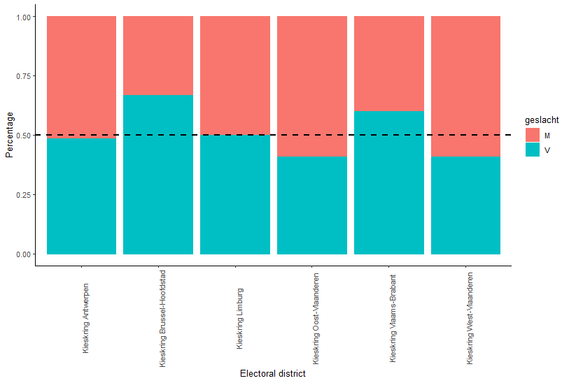
Again, we can answer some fun research questions with these data. For instance, is the share of women and men equal across electoral districts? We can create a plot to visualize the results.

plot2 <- ggplot(mp_bio_polinfo, aes(x = kieskring, fill= geslacht, colour = geslacht), bins = 12) + 
  geom_bar(position = "fill") +
  labs(x="Electoral district", y = "Percentage") + 
  theme_classic() +
  theme(axis.text.x = element_text(angle = 90)) +
  geom_hline(yintercept=0.50, linetype="dashed", 
             color = "black", linewidth=1)
plot2

Example 4 - ADVANCED: Extra unnesting of lists

The breadth of data available through the API is truly impressive. This also entails that we opted to return some data as nested lists (list of lists) storing multiple types of values. Yet, we are here to extract those values from these nested lists and construct a data frame ready for analysis. A great resource to learn about (un)nesting is here.

For this example, we analyze MPs accumulation of local political mandates. To obtain information about this, we start from the data frame mp_polinfo for which you filled in fact="political_info" in the get_mp() function. Next, we will unnest the column mandaat-andere containing the info about MPs other mandates. To do so, we use select() to only keep those variables/columns of interest and use unnest() to dig up information from the nested columns.

mp_polinfo %>%
  select(id_mp, naam, voornaam, mandaat_andere) %>%
  unnest(mandaat_andere) -> cumul
cumul

The data frame cumul now includes two new columns mandaatgroepnaam and parlmandaat. The latter column again being nested. So we still do not know the type of political mandate MPs hold at the local level. Are they a mayor, alder person or council member? To find out, we first filter out the local mandates using filter() on the column mandaatgroepnaam and then unnest()the column parlmandaat.

cumul %>%
  filter(mandaatgroepnaam == "Lokale mandaten") %>%
  unnest(parlmandaat) -> cumul_local
cumul_local

Next, we filter out the mandates MPs currently hold, leaving out former local functions by dropping all observations for which an end date (datumtot) is registered. Additionally, we also drop all other non-relevant columns using select().

cumul_local %>%
  filter(is.na(datumtot)) %>%
  select(id_mp, naam, voornaam, datumvan, mandaat) -> local_mand
local_mand

Finally, we create a new column in the data frame to register whether an MP holds a local function as mayor, alder person or council member. The column mandaat holds text (string values), we therefore recode this text into a new categorical numerical variable via an ifelse statement. To do so, we make use of the %like% operator to search through the text and identify who holds what local function.

local_mand$local_m <- ifelse(local_mand$mandaat %like% "burgemeester", 1, 
                                    ifelse(local_mand$mandaat %like% "schepen", 2, 
                                           ifelse(local_mand$mandaat %like% "gemeenteraadslid", 3, 4)))

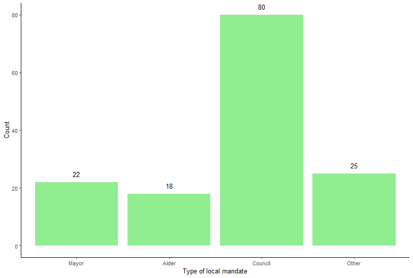
Let’s count how many MPs hold a local mandate.

n_distinct(local_mand$id_mp)

To visualize results, we make a plot.

plot3 <- ggplot(local_mand, aes(x = as.factor(local_m))) + 
  geom_bar(stat="count", fill="lightgreen") +
  geom_text(stat='count', aes(label=after_stat(count)), vjust=-1) +
  labs(x="Type of local mandate", y = "Count") +
  theme_classic() + 
  scale_x_discrete(labels=c("1" = "Mayor","2" = "Alder","3" = "Council", "4" = "Other")) 
plot3

Quick elaboration

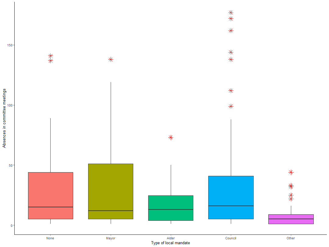
And we can again join this data frame with another data frame. For example, to answer the following question: Are mayors more frequently absent in parliament than other MPs?, we need to extract additional data about MPs presences in parliament (here: commissions). This can be done through filling in fact="presences_commissions" in the get_mp() function. Alternatively, you can choose to look at MPs presences in plenary sessions via fact="presences_plenary".

mp_commissions <- get_mp(selection="current", fact="presences_commissions")

We can then quickly explore these data to see which MPs are most often present/absent in the parliamentary committee sessions of which they are an effective member. We opted to focus on the top 10 most present/absent MPs (top_n(#, name column).

mp_commissions %>% select(id_mp, naam, voornaam, commissie_afkorting, commissie_id, `vast-lid-aanwezigheid_aanwezig`) %>% top_n(10, `vast-lid-aanwezigheid_aanwezig`) #present
mp_commissions %>% select(id_mp, naam, voornaam, commissie_afkorting, commissie_id, `vast-lid-aanwezigheid_afwezig`) %>% top_n(10, `vast-lid-aanwezigheid_afwezig`) #absent

To answer the question, we first select the relevant columns and then join the mp_commissions data frame with the local_mand data frame. We also exclude those observations that are not an effective member of a certain commission and therefore got assigned NA when registering their commission presences.

local_mand %>%
  select(id_mp, local_m) -> local_mand2

mp_commissions %>%
  select(id_mp, voornaam, naam, commissie_afkorting, commissie_id, `vast-lid-aanwezigheid_aanwezig`, `vast-lid-aanwezigheid_afwezig`, `vast-lid-aanwezigheid_verontschuldigd`) -> mp_commissions

Next, we implement a full_join of both the local_mand2 data frame and the mp_commissions data frame. Additionally, we assign the value ‘0’ to MPs holding no local mandate.

mp_m_comm <- full_join(local_mand2, mp_commissions, by=c("id_mp" = "id_mp")) 

mp_m_comm$local_m <- ifelse(is.na(mp_m_comm$local_m), 0, mp_m_comm$local_m)

mp_m_comm %>% 
  filter(!is.na(`vast-lid-aanwezigheid_afwezig`) & !is.na(`vast-lid-aanwezigheid_aanwezig`) & !is.na(`vast-lid-aanwezigheid_verontschuldigd`)) -> mp_m_comm_omit

Finally, we can visualize the results and conclude that mayors are not significantly more absent in commission sessions than other MPs. The data thus refutes the often heard claim that combining a local political mandate with a mandate in the Flemish parliament hampers parliamentary work.

plot4 <- ggplot(mp_m_comm_omit, aes(x=factor(local_m), y=`vast-lid-aanwezigheid_afwezig`, group=factor(local_m), fill=factor(local_m))) + 
  geom_boxplot(outlier.colour="red", outlier.shape=8, outlier.size=4) +
  labs(x="Type of local mandate", y = "Absences in committee meetings") +
  theme_classic() +
  scale_x_discrete(labels=c("0" = "None","1" = "Mayor","2" = "Alder","3" = "Council", "4" = "Other")) + 
  theme(legend.position = "none")
plot4